Passive sonar flowmeter technology — operating principles

Flow measurements in the mineral processing and mining industry suffer from the limitations placed by previously available flowmeters including the commonly used instruments such as ultrasonic meters, magmeters, turbine meters, orifice plate meters, vortex meters, Coriolis meters and Venturi meters. The desire or requirement to make a non-contact measurement that is accurate and robust, and can be performed on practically any type of fluid within practically any type of pipe, has driven the creation of a new class of flowmeters.

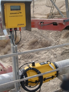
Utilising sonar-based processing algorithms and an array of passive sensors to measure naturally occurring sound in the process fluid, passive sonar flowmeters can measure not only flow, but also fluid composition. The result is a unique ability to measure the flow rate and entrained air level of most fluids — clean liquids, high solids content slurries, and liquids and slurries with entrained air. Sonar-based flowmeters are suitable for tracking and measuring the mean velocities of disturbances travelling in the axial direction of a pipe. These disturbances generally will convect with the flow, propagate in the pipe walls, or propagate in the fluid or slurry. First let us focus on the disturbances that convect with the flow. The disturbances that convect with the flow can be density variations, temperature variations or turbulent eddies. The overwhelming majority of industrial flows will have turbulent eddies convecting with the flow, thus providing an excellent means of measuring the flow rate as described below.

Turbulence

In most mineral processing processes, the flow in a pipe is turbulent. This turbulence occurs naturally when inertial forces overcome viscous forces.

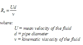
This turbulence can be expressed as the condition when the dimensionless Reynolds number, which is basically the ratio of the inertial forces over the viscous forces, exceeds approximately 4000. Below a Reynolds number of 2300, the flow is laminar, leaving the middle ground of 2300 to 4000 as a transitional flow regime containing elements of laminar and turbulent flow. The Reynolds number is given by:

As an example, a 200 mm pipe with water (or slurry with similar kinematic viscosity) flowing at 0.9 m/s (38.1 m³/h) at 20 °C has a Reynolds number of over 180,000 — clearly well above the criterion for turbulent flow.

Turbulent eddies and flow velocity

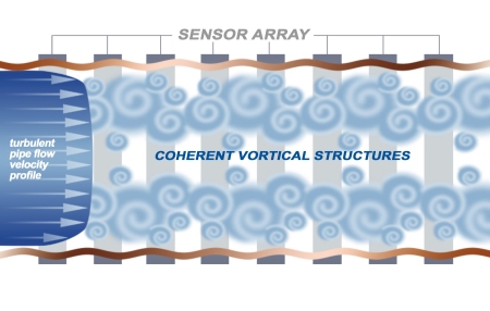
Turbulent flow is composed of eddies, also known as vortices or turbulent eddies, which meander and swirl in a random fashion within the pipe but with an overall mean velocity equal to the flow — that is, they convect with the flow. An illustration of these turbulent eddies is shown in Figure 1. These eddies are being continuously created, and then breaking down into smaller and smaller vortices, until they become small enough that through viscous effects they dissipate as heat. For several pipe diameters downstream, these vortices remain coherent, retaining their structure and size before breaking down into smaller vortices. On average, these vortices are distributed throughout the cross-section of the pipe and therefore across the flow profile. The flow profile itself is a time-averaged axial velocity of the flow that is a function of the radial position in the pipe with zero flow at the pipe wall and the maximum flow at the centre as seen in Figure 1. In turbulent flow, the axial velocity increases rapidly when moving in the radial direction away from the wall, and quickly enters a region with a slowly varying time-averaged axial velocity profile. Thus, if one tracks the average axial velocities of the entire collection of vortices, one can obtain a measurement that is close to the average velocity of the fluid flow.

Figure 1: Array measurement of flow velocity in a pipe with turbulent flow, showing fully developed flow profile and turbulent eddies.

Through the combination of an array of passive sensors and the sonar array processing algorithms, the average axial velocities of a collection of vortices can be obtained. The sequence of events to perform this measurement is as follows:

• The movement of the turbulent eddies creates a small pressure change on the inside of the pipe that results in a dynamic strain of the pipe wall itself (Figure 1 exaggerates).
• The mechanical dynamic strain signal is converted to an electrical signal through passive sensors wrapped partially or fully around the pipe.
• These sensors are spaced a precisely set distance from each other along the axial direction of the pipe, and a characteristic signature of the frequency and phase components of the turbulent eddies are detected by each element of the array of sensors.
• An array processing algorithm combines the phase and frequency information of the sensor array elements to calculate the velocity of the characteristic signature as it convects under the array of sensors.

The challenges of performing this measurement in a practical manner are many. These include the challenges of operating in an environment with large pumps, flow-generated acoustics and vibrations, all of which can cause large dynamic straining of the pipe. The impact of these effects is that the dynamic strain due to the passive turbulent eddies is usually much smaller than the dynamic strain arising from pipe vibrations and acoustic waves propagating in the fluid. The strength in the array processing algorithm is its ability to isolate and measure the velocities of these different components, including the weak signal from the convecting turbulent eddies and the strong signals from the acoustic waves and vibrations.

The algorithm processes the signals from the sensor array elements to deconvolve the frequency and length scale components. Each wave number, which is the inverse of the corresponding length scale component, is analysed to determine the energy contained in its frequency spectrum. The peak energy in this frequency spectrum occurs at a frequency point given by:

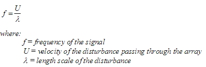
When performed over the entire range of desired wave numbers, a plot of this energy distribution called a k-ω plot (k=2π/λ) and ω=2πf) is generated with the x-axis defined by the wave number (1/ λ) and the y-axis defined by the frequency (f).

By rearranging the previous equation we obtain: This is basically the slope of the energy distribution. Figure 2 allows us to readily see how every point on the peak energy ridge contributes to the velocity measurement. In this example, the amplitude shown in the graph is on a log scale, so the peak energy is about 15 dB higher than the energy next to the ridge and about 25 dB higher than the other energy regions seen in the graph. The resulting slope of the ridge formed by these peak energy points is equal to the average velocity of the passing disturbance, which in this case is the passing turbulent eddies or vortices.

Figure 2: A representative k-ω plot showing convective ridge.

The technology can also generate an indication of the robustness of the measurement, otherwise known as a quality factor. Typically, flowmeters do not provide an indication of the quality of the measurement, but in the sonar processing algorithm such a quality factor can be generated by comparing the strength of the ridge against background energy levels. A quality factor ranging from 0 to 1.0 is generated, with any flow measurement providing a quality factor above 0.1 to 0.2 (depending on the application) being considered to be a good measurement.

Currently, this technology can report the volume flow rate on liquids and slurries with flow velocities extending from one to several hundred metres per second. The technology lends itself to measurement on practically any pipe size, as long as the flow is turbulent, and for some non-Newtonian fluids, even without turbulence. The pipe must be full but it can have entrained air in the form of well-mixed bubbles.

Array measurement of acoustic waves

As mentioned earlier, the same sensors and algorithm can be used to measure the velocity of naturally occurring acoustic waves that are travelling in the fluid. This fluid can be multiphase, or multi-component single phase. In a single-phase mixed fluid, the acoustic velocity is a function of the ratio and acoustic properties of the two fluids, thus this measurement can be used to determine mixture ratios through application of the simple mixing rule (volume average of velocity). The resulting acoustic velocity c_M can be given by:

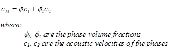
Using Φ₂ =1-Φ₁ this can be rearranged to give:

In multiphase fluids that consist of a gas mixed with a liquid or slurry, the acoustic velocity can be used to determine the amount of entrained gas (gas void fraction) when the gas is in the form of bubbles that are well mixed within the liquid or slurry.

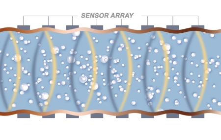
These acoustic waves are generated naturally from a variety of sources, including pumps, flow-through devices and flow-through pipe geometry changes. These acoustic waves are low frequency (in the audible range), travel in the pipe’s axial direction and have wavelengths much longer than the entrained gas bubbles. An illustration of these acoustic waves in a pipe is shown in Figure 3 and they can propagate in either direction down the pipe or in both directions. Since acoustic waves are pressure waves, they will dynamically strain the pipe during the cycling from compression and to rarefaction and back. This dynamic strain is then captured by the sensors and converted to an acoustic velocity measurement.

Figure 3: Naturally occurring acoustic waves propagating in a pipe under the sonar array sensors.

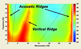
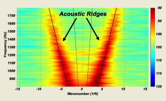
A representative k-ω plot of a hydrocyclone feed line with entrained air is shown in Figure 4. Here one can see the vortical ridge and the acoustic wave ridges on the left graph.

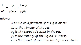
By rescaling the graph and looking at higher frequencies, a better view of the acoustic ridges is obtained. Since the wavelengths of the acoustic waves are much larger than the bubble size, a complex interaction takes place that sets the acoustic velocity to be a strong function of the gas void fraction. In this case, the relationship is expressed with Wood’s equation. The speed of sound is proportional to the square root of the ratio of the compressibility and the density. The mixture compressibility equals the volumetrically averaged compressibility of the two separate components. The mixture density follows a similar relationship in which it equals the volumetrically averaged density of the two separate components. The resulting equation is given by: and		Figure 4a: A k-ω plot showing both acoustic ridges and vortical ridge.
		Figure 4b: Rescaling of the graph and a change in frequency range enhances the view of the acoustic ridges.

By solving for Φ and taking into account the compliance of the pipe, the acoustic velocity or speed of sound can be converted to a phase fraction of gas (gas void fraction). An example of the resulting relationship is shown in Figure 5.

Figure 5: Example of the relationship between gas void fraction and speed of sound.

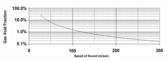
The gas void fraction measurement is used in a variety of different fields and applications. Within minerals processing, it is used for nuclear density gauge correction, flowmeter correction to provide true volume flow and air injection applications. It has been successfully used for entrained air applications ranging from 0.01% to 20% gas void fractions with an accuracy of 5% of the reading.

Proven technology

Sonar-based flow instruments have been installed in over 11 countries and have proved themselves in grinding and classification, refining, leaching and smelting operations. These include hydrocyclone feed, overflow and underflow lines, water feed and recovery lines, SAG mill and ball mill discharge lines, thickener underflow lines, tailings lines, final concentrate lines, red mud and green liquor bauxite lines, pregnant leach solution lines, raffinate lines, organic lines, acid lines and scrubber water lines.

In many of the minerals processing and mining industries, it is the only technology able to provide reliable flow and gas volume fraction measurement.

Krohne Australia
www.krohne.com